
* Although radars went through a rapid evolution during World War II, the rate of change in the technology leveled out in the postwar period. The pace picked up again in the 1960s with the introduction of solid-state and digital technology -- in particular leading to the development of the "pulse Doppler" radar, which finally managed to solve the problem of ground clutter.
* The schemes for angle tracking a target discussed so far -- lobe switching and conical scan -- have a limitation. As mentioned, the RCS of a target may vary dramatically from one moment to the next. If, say, lobe switching is used by a radar tracking a target, then the radar return may change amplitude drastically from one pulse to the next. The tracking system will think it is losing track on the target when it really isn't, breaking tracking lock.
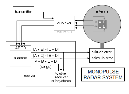
The answer to this difficulty is obvious in hindsight: send multiple pulses on angular offsets at the same time. Suppose a radar transmitter antenna has two feed horns, each slightly offset from the antenna boresight. This arrangement allows two pulses to be sent at the same time, with the returns from both pulses being picked up by the receiver subsystem at the same time. The radar tracking system will be handed both the sum and the difference of these two returns, and will then rotate the antenna to ensure that the sum remains at a maximum and the difference remains at a minimum. This is known as "monopulse" operation.
Obviously, as described above this scheme only tracks a target along one axis. In practice, a monopulse system will have four feed horns to track a target along both axes.
A scheme was once used that involved twin feed horns with conical scanning, and was not surprisingly known as "conopulse". It was tricky to do, and is now generally out of use.
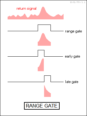
* Another technique developed in the postwar period was "range tracking", in which the radar automatically kept track of the distance to the target. This was done by using a "range gate" technique, in which the radar system kept track of, or "sampled", the target echo on the radar return trace between traces. The sampled return signal was further monitored by halves with an "early gate" and a "late gate". The relative energy of the return signal in the two half-gates was then used to adjust the position of the "main" gate to keep a range lock on the target.
* Automatic tracking schemes by radar implied that the radar has some ability to interpret the return trace on its own. In early radars, as mentioned earlier all the radar did was display the return trace to the radar operator, and the radar operator had to interpret it -- picking the target out of noise and estimating its range, direction, speed, and size. This made radar operation something of an art, but people are adaptable and radar operators could become very "artistic" in their ability to read the radar display. The push in modern radars has been to eliminate the need for interpretation, using electronic smarts to duplicate the abilities of the human brain.
BACK_TO_TOP* In the postwar period, the magnetron gradually gave way to two microwave vacuum amplifier tube technologies, the "klystron" and the "traveling wave tube (TWT)". It was difficult to scale up magnetrons to very large size, and new radar systems also began to demand a level of frequency stability that a magnetron couldn't private. The magnetron didn't go away, since it is cheap and efficient, and it still remains in widespread use in microwave ovens. According to legend, the microwave oven was invented by a radar engineer who stood too close to a magnetron and found out that a chocolate bar in his pocket had melted.
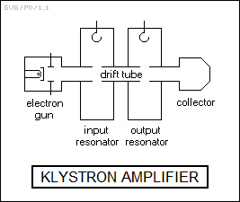
The klystron actually more or less predates the magnetron, having been invented by the Varian brothers in 1939, but it took longer to turn into a really useful device. In a simple klystron, an electron beam is generated by a heated cathode, to be shot through a ring-style anode down a "drift tube" towards a secondary anode called the "collector". The drift tube passes through two resonant cavities, one for signal input and one for signal output, with the tube broken by an "interaction gap" in each cavity. In the input cavity, the input signal modulates the electron beam passing down the drift tube, and when the modulated signal reaches the output cavity, it dumps RF energy into it, to be tapped off to the external system.
As with magnetrons, there is wide variation in klystron configurations, for example klystrons with multiple cavities. It is also possible to build a "reflex klystron" oscillator tube that replaces the collector with a plate that reflects the electron beam back into a single resonant cavity.
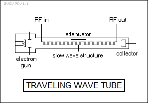
* A klystron is efficient and can be scaled up to very large size, but it can only amplify signals over a relatively narrow bandwidth. In contrast, the TWT can amplify signals over a wide bandwidth. The TWT was invented in 1943, but didn't really come into its own until well after World War II. Like the klystron amplifier, the TWT has an electron gun system that shoots an electron beam down towards a collector. However, instead of a resonant cavity, the TWT has a long metal spiral or helix assembly, known as the "slow wave structure", through which the electron beam passes. The RF input signal is linked to the entrance of the slow wave structure, and the influence of the input signal causes the electron beam to "bunch up" at the same frequency. This results in considerable amplification of power, which is tapped off the exit of the slow wave structure. The electron flow through the slow wave structure has to be confined by a magnetic field from an external coil or permanent magnets to keep it focused. A grid can be inserted into the flow path to shut the beam on and off.
Such a "helix" TWT has the limitation that it doesn't work well for high power output; a high average power output means a high electron flow through the tube that heats up the helix, and getting rid of the heat becomes tricky. High peak powers imply increasing the speed of the electron flow, which means stretching out the helix, up to the point where it is spaced so widely that it can't modulate the beam any longer. As a result, other slow wave structures are used in high power TWTs, for example a series of coupled cavities.
Of course, the klystron and TWT are only used for the high-power output stages of a radar. In the early postwar period the rest of the system was run by ordinary vacuum tubes, with these systems gradually upgrading to more compact, less power-hungry, and more reliable solid-state transistor technology in the late 1950s. The introduction of solid-state devices led to integrated circuits (ICs), which gave radars much more sophisticated capabilities.
There was a belief decades ago that high-power microwave transistors would soon reduce klystrons and TWTs to obsolescence, but the older technologies remain alive and well for the time being. Klystrons and particularly TWTs are reliable, efficient, and cost-effective -- though it appears that semiconductor devices are gradually putting them out of business.
BACK_TO_TOP* So far, all the radars discussed in this document use a mechanically-steered antenna. It is also possible to steer a radar beam electronically. Imagine a transmitting antenna made up of a number of dipoles in a row; the beam could be shifted to the left by increasing the phase of the output waveform from the right side to left side of the array of dipoles; and to the right by decreasing the phase from the right to left side. This is known as "electronic steering" or "phased array". A phased array may also have additional mechanical steering -- for example, using mechanical steering in altitude and electronic steering in azimuth.
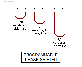
There are a number of ways of achieving the phase shift. One of the conceptually simplest is to use "programmable phase shifters". Each phase shifter consists of a set of switches that can be set to provide a direct connection, or a connection through a delay line. A typical configuration would use three switches, one with a delay line providing a phase shift of half a wavelength / 180 degrees; the second with a delay line providing a phase shift of a quarter wavelength / 90 degrees; and the third with a delay line providing a phase shift of an eighth of a wavelength / 45 degrees. This scheme can produce any phase shift from 0 to 315 degrees in increments of 45 degrees.
A simple phased array radar uses a central oscillator, with its output fed to a set of phase shifters, each connected to a single antenna element. As is generally the case for antennas, operation of a phased-array antenna is reciprocal: the phase shifters bring the return from a target back into phase for detection. A phased array can generally provide a field of view about 120 degrees across -- for 360 degree coverage, three arrays are mounted on a triangular base -- and it can switch beam position in microseconds. Phased array techniques can also be used to vary the shape of the beam, a scheme known as "digital beam forming".
Another approach to phased array operation that was used on some big radars -- such as the huge and well-known fixed-antenna "billboard" radars at the Ballistic Missile Early Warning System (BMEWS) radar sites in Alaska and Greenland, built in the early 1960s -- achieved beam steering by switching between different sets of feed horns. This "organ pipe" scheme didn't give much pointing accuracy, but for a broad-beam surveillance radar, such accuracy wasn't needed anyway.
The disadvantage of a phased-array radar is that it means substantially greater complexity, at least traditionally raising cost and bulk. Phased array radars have tended to be the exception and not the rule, useful for specialized applications where cost is not such an obstacle. Modern technology is lowering the cost and increasing the utility of phased arrays.
Phased-array radars have a certain "whizzy" flavor to them, but they are conceptually nothing new. They were originally developed by both the Americans and the Germans in World War II, using electromechanical switching schemes for the phase shifters. Of course, their switching speeds were much lower than those for modern phased-array radars, and comparing the World War II phased-array radars to a modern phased-array radar is like comparing a World War I Sopwith Camel fighter to an F-16 jet fighter.
BACK_TO_TOP* One of the particularly troublesome issues with early radars was clutter. Early ASV and targeting radars, as mentioned, could only perform gross discrimination between targets, and clutter could be a problem for air surveillance radars as well -- for example, a ground-based radar would pick up reflections from nearby ground clutter at low angles of altitude. The simplest way to deal with the problem was to keep the receiver turned off until the radar pulse has "cleared" the ground clutter, but this also left the radar completely blind at ranges shorter than that.
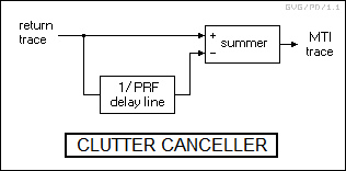
An improved scheme was developed that wasn't that much more complicated: simply store a return trace in a "delay line" for the pulse period, then get a second return trace and subtract the first trace from it, eliminating the parts that didn't change. Anything that hasn't moved between the two traces, meaning the ground clutter, will more or less disappear, while anything that moves between the two traces, meaning the target, will remain. This was called a "clutter canceler", with the overall system referred to as a "moving target indicator (MTI)".
Simple MTI using analog technology is a straightforward idea, but it's not very sophisticated; it results in a signal that's noisy and difficult to interpret. A more sophisticated scheme is the "Ground Moving Target Indicator (GMTI)", discussed below.
* One of the problems with MTI as described is that it won't work if the radar platform is moving, since then the clutter returns will be very different from pulse to pulse and won't cancel out.
A trick was developed that could be used to make a radar carried in an aircraft look like it is standing still, at least from one pulse to the next. Suppose an aircraft has two radar antennas in tandem and is taking radar observations to the side of the aircraft flight track. The leading antenna emits a pulse, then advances forward and picks up the return. When the trailing antenna reaches the position where the leading antenna was when it emitted its pulse, the trailing antenna emits its own pulse, and then advances to pick up the return in the same position as did the leading antenna. This gives two pulses and returns obtained in the same location, allowing a clutter canceler to be used to compare them to find moving targets.
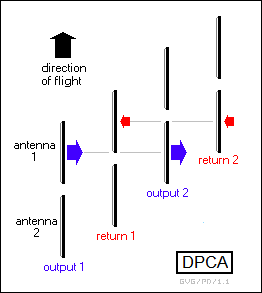
This was given the name of "displaced phase center antenna (DPCA)". As defined, it is complicated and tricky to implement, particularly since the PRF of the radar has to be readjusted precisely with changes in aircraft flight speed. In practice, the same principle could be used with much more sophisticated processing, for example using a single rotating antenna with a beam shifted slightly from one side to the other.
BACK_TO_TOP* The full answer to the problem of clutter was the development of the "pulse Doppler" radar, hinted at earlier, which can obtain range data by timing radar returns, and velocity data by measuring the Doppler shift of the returns. However, a pulse Doppler radar is much more sophisticated than a simple pulse radar, and a little additional theory is required to understand its operation.
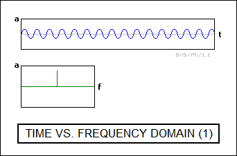
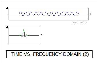
The first item is to introduce is the concept of "time domain" versus "frequency domain". According to a branch of mathematics known as "Fourier analysis", any time-varying signal, no matter how complicated, can be broken down into a set or "spectrum" of simple pure sine waves of different frequencies, amplitudes, and phases. A "Fourier transform" can be used to convert the "time domain" signal into a "frequency domain" spectrum, while an "inverse Fourier transform" can be used to convert the frequency domain spectrum into a time domain signal.
The exact details of performing a Fourier or inverse Fourier transform are beyond the scope of this document. The reader can simply imagine having an electronic box that displays a time-domain waveform, such as a radar return trace, and then with a push of a button displays the frequency spectrum of that radar return. Such a device is called a "spectrum analyzer". It must be emphasized that a spectrum analyzer is not a component of a radar system, though it might be used to help develop or troubleshoot one, it's just used here as a tool to visualize and deal with the relationship of a time-domain waveform and a frequency-domain spectrum. They're two sides of the same coin; some things that are hard to see in the time domain can be very obvious in the frequency domain, and the reverse.
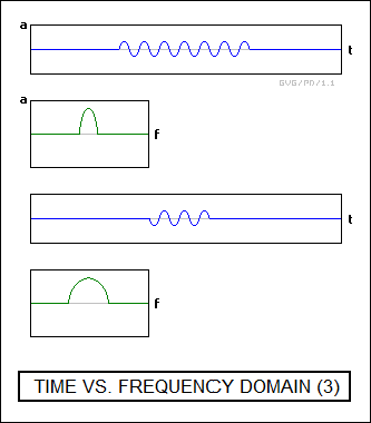
In the simplest case, let's use the spectrum analyzer to observe the output of a simple CW Doppler radar, ignoring the return. The frequency-domain plot, the spectrum, is simple and obvious: there's one line at the radar carrier frequency.
This assumes that the carrier signal is continuous. Suppose this carrier signal is actually turned on at one time and then turned off at another, turning it into a very long pulse. This changes the spectrum slightly: instead of a nice neat line at the carrier frequency, the spectrum acquires the form of a heavily damped sine wave, with a peak centered on the carrier frequency and the cycles or "lobes" of the sine wave fading rapidly to each side of the spectrum. This spectrum follows the form of the SIN(X)/X or "sinc" function.
Fourier analysis assumes that all the component sine waves making up a time-domain signal are continuous; that means a range of sine waves of different amplitudes, frequencies, and phases are present, but interfere with each other in such a way so that the time-domain function cancels out at the ends of the pulse. It can be simply stated as a given that the spectrum required to do this follows the sinc curve; explaining why would be more trouble than it would be worth here. Anyway, the central mainlobe of the sinc curve is much larger than all the sidelobes, and so as a useful simplification the sidelobes can be ignored, reducing the function to the mainlobe.
Now suppose we start cutting the interval between turning the pulse on and off in half. With every reduction in pulse width by a factor of two, the width of the mainlobe doubles. This is because the smaller the pulse, the broader the range or "bandwidth" of sine-wave components required to squeeze it into its desired length. The relationship can be expressed with the simple rule-of-thumb:
mainlobe_bandwidth = 2 / pulse_width
In other words, for a pulse width of a microsecond, the mainlobe bandwidth will be 2 MHz. Go to two microseconds, it will be 1 MHz.
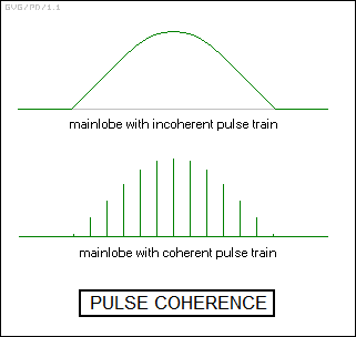
Next, instead of producing a single pulse, we start producing a train of pulses at a given PRF. At first, it doesn't seem to make any difference: the mainlobe spectral plot looks exactly as it did with a single pulse. It is impossible to perform any sort of Doppler processing on a simple pulsed radar, since the Doppler frequencies will be much closer to the center frequency than the ends of the mainlobe band, remaining buried inside the mainlobe spectrum, with no way to pick them out. In other words, the normal variation in frequency of the signal due to its spectrum of components covers a continuous range that masks out any variations due to Doppler shifting.
The problem with this simple pulsed radar scheme is that the pulses are "incoherent", meaning that the phase of one pulse has no continuity with any previous pulses. To fix the problem, we can generate a train of "coherent" pulses instead. This can be done by generating a continuous carrier signal and a separate pulse train, and then using the pulse train to "gate" the continuous carrier signal to the output of the radar; such a system is known as a "stable local oscillator (STALO)". From the point of view of the Fourier transform, this simplifies the spectrum considerably. Instead of the continuous mainlobe, the result is a set of distinct spectral lines, spaced at regular intervals but with the amplitudes of the lines following the envelope of the mainlobe curve.
That means that a pulsed "coherent" radar can perform Doppler processing. However, there's a catch. Suppose we start increasing the PRF. The result is that the spectral lines start moving apart; as it turns out, the spacing of the spectral lines is defined by the PRF. For a PRF of 5,000 Hz, the spectral lines are 5,000 Hz apart; for a PRF of 1,000 Hz, the spectral lines are 1,000 Hz apart.
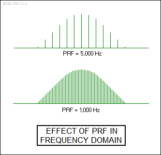
With a simple pulse radar, a low PRF / long pulse interval is useful to eliminate range ambiguities and ghosts. However, from the point of view of Doppler processing with a pulsed coherent radar, a low PRF means that the spectral lines are spaced closely together, making it very difficult to pick out Doppler frequencies in the returns. If the Doppler-shifted return has exactly the same frequency as one of the lines in the transmit spectrum, there will be no way to detect the "blind speed". If the Doppler-shifted return has a frequency greater than that of the line above the transmit line that actually produced it, it will give an ambiguous velocity; as will a Doppler-shifted return with a frequency lower than the line below. This is something of a frequency-domain "mirror" of the blind zones and range ambiguities, discussed previously for simple pulse radars.
In other words, a low PRF results in little range ambiguity, but troublesome Doppler ambiguities. A high PRF results in exactly the opposite situation: little Doppler ambiguity, but troublesome range ambiguities. Of course, it is possible to get the best of both worlds by using a "pulse burst" scheme, with the transmitter sending out pulses on a long interval to get range, and interleaving sets of short-interval pulses to get velocity.
Incidentally, detecting the phase of the return signal relative to the coherent output pulse requires that two returns be obtained: one that is the result of a direct comparison with the coherent output signal, and so is known as the "in phase (I)" signal; and one that is the result of the coherent output signal shifted 90 degrees, and so is known as the "quadrature (Q)" signal. The magnitudes of the I and Q signals at each instant have to be compared to give the relative phase change.
* Pulse Doppler radar didn't really become practical until the late 1960s, with the introduction of digital technology to radars. Instead of trying to come up with sets of analog electronic circuits, each one dedicated to a specific task, the return could be "digitized" into a set of numeric values, allowing a computer to be used to control the radar -- juggling the transmit waveforms, manipulating the returns, and interpreting the results for the user.
Very significantly, a computer can perform a Fourier transform on a signal converted to a digital form. This is known as a "discrete Fourier transform (DFT)", or more informally a "digital Fourier transform". In any case, a basic DFT can be optimized to make the calculations more economical and faster, resulting in a "fast Fourier transform (FFT)". This means that a computer can take an echo returned by a radar, perform an FFT on it, and then sort out all the spectral "components" by their different frequencies. This not only allowed the computer to sort out chaff from target echoes, it also allowed the radar to sort out and discard ground clutter as well -- a scheme known as "notching" -- eliminating the clumsy dual-antenna scheme of AMTI.
A modern pulse Doppler radar can in principle operate in multiple modes. In the "low PRF" mode, the radar can obtain unambiguous ranges at the expense of highly ambiguous Doppler velocities. In the "high PRF" mode, the radar can obtain unambiguous velocities at the expense of highly ambiguous ranges, though FM ranging, with successive pulses emitted at increasing frequencies in a "ramp" pattern, can be used to reduce the ambiguities. In a "medium PRF" mode, the radar achieves a compromise between the two. To reduce ambiguities, the radar can perform "PRF jittering", sending out a pulse on one interval, followed by a pulse on a different interval, then a pulse on yet another different interval, until it finally goes back to the original interval and begins the cycle again.
BACK_TO_TOP* It is useful to discuss some other interesting features of modern radars before proceeding further. One is the concept of the "range bin", which allows automated range tracking of targets and the ability to pick targets more easily out of noise.
Range bins are a scheme in which a digital radar uses a set of range gates to chop up the return trace into segments and sum the value for each segment into an associated in a memory "bin". The radar system can inspect the bins to see where the target is along the trace and track its range, but it can also sum up values from trace to trace relative to an average level. Since noise will tend to fluctuate around the average level, the contents of most of the range bins will remain at the average level. The radar system can keep track of the average noise level in the range bins and adjust the noise threshold accordingly, a scheme known as "constant false alarm rate (CFAR)". If there is a return signal in a range bin, it will tend to add up over time, making it easier to pick out of the noise. If the signal shows up in two or more adjacent bins, the radar can also interpolate between the two to get a more accurate range estimate.
This is shown in the diagram below, which displays the summing of eight return traces in a set of eight range bins. Digitizing a waveform means it is resolved into a discrete set of values or steps; this diagram uses the simplifying assumption that the values of each trace are very close to the noise level and only have values of a single step above, at, or below the average signal value level, which is shown in gray. Of course, in reality they may vary several steps above or below the average signal value.
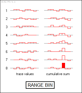
Apparently much the same technique could be used in sophisticated analog radars, with a range bin value stored by an "integrating filter" that could add up analog signals. However, the digital range bin approach has replaced such schemes.
* Another modern improvement is known as "pulse compression". As was shown in the description of simple pulse radars, there is a trade-off in determining pulse width. A short pulse gives better range accuracy, but it also means less energy dumped out to sense a target. Pulse Doppler makes the matter worse: interpreting the Doppler shift from a short pulse is harder than interpreting the shift from a long pulse, and so a short pulse gives poorer velocity resolution.
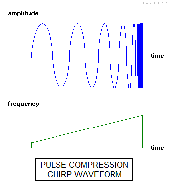
The answer is pulse compression. In the simplest form, it amounts to generating the pulse as a frequency-modulated ramp or "chirp", rising from a low frequency to a high frequency. This increases the energy of the pulse (wave energy increases with frequency) and permits much less ambiguity in Doppler interpretation. Essentially, pulse compression trades bandwidth for pulse length, and pulse compression schemes are rated by a "compression factor" given by:
compression_factor = chirp_range * pulse duration
There are also "coded" schemes for pulse compression that involve shifting parts of the pulse in phase. For example, consider a simple sine wave, going through cycle after cycle, with each cycle consisting of the signal going from zero amplitude to a positive value back through zero to a negative value and back to zero again. A normal sine wave will go through identical cycles in sequence, varying from positive to negative through each cycle.
Now suppose, say, that every third cycle the sine wave is inverted in polarity, varying from negative to positive instead of positive to negative, or in other words shifted 180 degrees in phase:
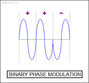
The three-part pattern of unshifted and shifted cycles can be described in a simple shorthand as a type of "binary code", with values of "+" (unshifted) and "-" (shifted). In this case, the code is given by:
+ + -
In any case, by Fourier analysis the abrupt transition from a "+" cycle to a "-" cycle involves a very wide spectrum of Fourier components, and so by the seemingly simple change of inverting one cycle of polarity results in a compressed high-bandwidth pulse generated from a relatively low-bandwidth signal. Of course, the received return pulse is processed by summing the echoes obtained from the three pulses, with the third cycle returned to normal polarity in the summation. This, by a bit of signal processing magic, gives an energetic return even with a short pulse.
The details of how pulse coding is implemented and actually works are far beyond the scope of an elementary discussion of radar. There are various types of coding sequences, each with somewhat different properties, and some use other phase shifts than 180 degrees. This description does no more than introduce the concept for further study elsewhere.
BACK_TO_TOP