
* This chapter provides basic definitions of and introductory concepts for radar technology.
* Radar is a variant of radio technology and shares many of the same basic elements. It is useful to discuss fundamental concepts of radio operation to provide a basis for discussing fundamental concepts of radar operation.
Late in the 19th century, researchers discovered that if an alternating electric current were run through a wire or rod, it emitted an invisible form of radiation that could generate an alternating electric current in a remote wire or rod -- with no wired electrical connection between the two. This invisible radiation was quickly realized to be a form of "electromagnetic (EM) radiation", a disturbance of electric and magnetic fields that propagated through space.
Electromagnetic radiation is in the form of waves propagating at a speed of 300,000,000 meters per second (186,000 miles per second). The waves could be generated at varying "frequencies", defined by the number of cyclical variations of the wave that passed every second through a plane perpendicular to the motion of the wave. Frequencies were once measured in "cycles per second (CPS)", but now are universally defined in terms of "hertz (Hz)", after Heinrich Hertz, a pioneering radio researcher.
The frequencies of electromagnetic radiation are usually large numbers, and so it is useful to use "metric prefixes" as shorthand. For example:
   kilohertz (kHz):   1,000 hertz
   megahertz (MHz):   1,000,000 hertz
   gigahertz (GHz):   1,000,000,000 hertz
   terahertz (THz):   1,000,000,000,000 hertz
The full range of frequencies of EM radiation is known as the "electromagnetic spectrum". Radio waves only take up part of this spectrum, in practice generally in the form of kilohertz, megahertz, or gigahertz radio emissions. Above about 300 GHz, EM radiation moves into a region of the spectrum known as "infrared"; and then with increasingly higher frequencies (and incidentally, higher energies) into the region of visible light that we can see with our eyes; and finally into energetic radiation defined as the "ultraviolet", "X-ray", and (at the very highest frequencies) "gamma ray" regions of the spectrum.
Put more simply, radio waves are the same thing as visible light, both being forms of EM radiation. The only real difference is that radio waves have lower frequencies. Incidentally, electromagnetic waves are entirely different from sound waves, which are mechanical disturbances propagating through the air, water, or a solid medium. The two kinds of waves can be confused because very low frequency EM waves are sometimes said to be at "audio" frequencies, matching the frequencies of the sound waves we can hear, and of course EM waves can be used to transmit audio, as turning on a household radio receiver shows.
* This document focuses only on radio waves. Sometimes it is easier to talk about radio waves in terms of their "wavelength" in meters instead of their frequency. There is a simple relationship between the wavelength and frequency of a wave:
wavelength = 300,000,000 / frequency
-- where 300,000,000 is the propagation speed of EM radiation in free space in meters per second. If frequency and wavelength are given in the appropriately scaled units of measurement -- kilohertz and kilometers, megahertz and meters, or gigahertz and millimeters -- this simplifies to:
wavelength = 300 / frequency
The list below gives the wavelengths at various frequencies:
     1 kHz = 300 kilometers
     3 kHz = 100 kilometers
    10 kHz = 30 kilometers
    30 kHz = 10 kilometers
   100 kHz = 3 kilometers
   300 kHz = 1 kilometer

     1 MHz = 300 meters
     3 MHz = 100 meters
    10 MHz = 30 meters
    30 MHz = 10 meters
   100 MHz = 3 meters
   300 MHz = 1 meter

     1 GHz = 30 centimeters
     3 GHz = 10 centimeters
    10 GHz = 3 centimeters
    30 GHz = 1 centimeter
   100 GHz = 3 millimeters
   300 GHz = 1 millimeter
Frequency and wavelength are two sides of the same coin, with frequency being a useful term in some cases and wavelength being more convenient in others. This document switches back and forth between them at will.
Various frequency / wavelength ranges, or "bands", have been defined for radars, with general classes of equipment usually operating in one or a few bands. The band names as defined by the International Telecommunications Union (ITU), an electronic standards body, with the frequency / wavelength corresponding to the lower or base end of each band, are as follows:
   ___________________________________________________________________

   ELF (Extremely Low Frequency)  30 Hz      10,000 kilometers
   VF  (Voice Frequency)          300 Hz     1,000 kilometers
   VLF (Very Low Frequency)       3 kHz      100 kilometers
   LF  (Low Frequency)            30 kHz     10 kilometers
   MF  (Medium Frequency)         300 kHz    1 kilometer

   HF  (High Frequency)           3 MHz      100 meters
   VHF (Very High Frequency)      30 MHz     10 meters
   UHF (Ultra High Frequency)     300 MHz    1 meter

   L                              1 GHz      30 centimeters
   S                              2 GHz      15 centimeters
   C                              4 GHz      7.5 centimeters
   X                              8 GHz      3.75 centimeters
   Ku                             12 GHz     2.5 centimeters
   K                              18 GHz     1.67 centimeters
   Ka                             27 GHz     1.1 centimeters

   V                              40 GHz     7.5 millimeters
   W                              75 GHz     4 millimeters
   mm                             110 GHz    2.73 millimeters
   ___________________________________________________________________
The VLF through UHF band definitions were inherited from radio engineering. The band names above UHF don't follow any apparent logical pattern, which was apparently done by intent, as a military security measure. The K band originally also included the Ku and Ka bands, but it turned out that the center portion of the K-band was useless for most military purposes -- since water vapor in the atmosphere soaked up and blocked radio waves in that range. The portion of the K-band "above" the absorption range became the "Ka-band", while the portion "under" the absorption range became the "Ku-band". About the only way to remember the order of these bands is with a mnemonic, for example: "Lincoln State College eXplorer's Kit". Gear operating in the V and W bands is usually just referred to as "millimeter wave".
To make things more confusing, different band definitions are used in other electronic fields. Radio engineers retain the ELF through UHF definitions, but take the UHF band up to 3 GHz, and then cover the higher frequencies with the "Super High Frequency (SHF)" band from 3 to 30 GHz, covering the centimetric / microwave region; and then the "Extremely High Frequency (EHF)" band from 30 to 300 GHz:
   ___________________________________________________________________

   ELF (Extremely Low Frequency)  30 Hz      10,000 kilometers
   VF  (Voice Frequency)          300 Hz     1,000 kilometers
   VLF (Very Low Frequency)       3 kHz      100 kilometers
   LF  (Low Frequency)            30 kHz     10 kilometers
   MF  (Medium Frequency)         300 kHz    1 kilometer

   HF  (High Frequency)           3 MHz      100 meters
   VHF (Very High Frequency)      30 MHz     10 meters
   UHF (Ultra High Frequency)     300 MHz    1 meter

   SHF (Super High Frequency)     3 GHz      10 centimeters
   EHF (Extremely High Frequency) 30 GHz     1 centimeter
                                  300 GHz    10 millimeters
   ___________________________________________________________________
There is also a completely different NATO band scheme, with the bands much more conveniently arranged from "A" to "M" in order of increasing frequency. There isn't a one-to-one correspondence between the NATO and traditional band schemes. The table below gives the NATO bands, with the frequency / wavelength given in each entry for the low end of the band:
   ___________________________________________________________________

   A        0 Hz         -
   B        250 MHz      1.2 meters
   C        500 MHz      60 centimeters
   D        1 GHz        30 centimeters
   E        2 GHz        15 centimeters
   F        3 GHz        10 centimeters
   G        4 GHz        7.5 centimeters
   H        6 GHz        5.0 centimeters
   I        8 GHz        3.75 centimeters
   J        10 GHz       3.0 centimeters
   K        20 GHz       1.5 centimeters
   L        40 GHz       7.5 millimeters
   M        60 GHz       5 millimeters (up to 100 GHz / 3 millimeters)
   ___________________________________________________________________
The NATO band scheme seems to be more popular in Europe, and is used worldwide for "electronic countermeasures" systems -- that is, radio / radar jamming gear. In some publications it can be very unclear which scheme is being used, which can be very confusing since the ITU and NATO schemes share some of the same designation letters, applied to entirely different ranges -- for instance, there are "C", "L", and "K" bands in both schemes that don't have the matching definitions. Fortunately, the NATO scheme ends at "M", so "S" and "X" bands can always be recognized as ITU definitions -- as can the "Ku" and "Ka" bands, since the NATO bands are all one letter. Since there's no clear standard, this document uses the ITU band definitions.
BACK_TO_TOP* Since electromagnetic radiation is a wave phenomenon, it has certain characteristics associated with waves, such as "polarization", "phase", and "wave interference".
The oscillations of an EM wave occur back and forth across the direction of the wave's propagation. This means that the wave has a certain "polarity". If the wave's oscillations are up and down, the wave is said to be "vertically polarized"; if they are left and right, the wave is said to be "horizontally polarized". Of course, the wave could also be polarized at any angle between those two extremes.
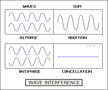
The concepts of "phase" and "wave interference" are a bit trickier to explain. Imaging a tank of water with some sort of vibrating element to generate waves stuck into it. If another vibrating element is stuck into the water operating at the same vibration rate and same intensity, it will generate waves of the same frequency and height (or "amplitude"), but the peaks and valleys of the waves generated by the second vibrating element will not necessarily coincide with those of the first. In other words, they won't have the same "phase".
The phase of the two sets of waves could be matched up, with the peaks and valleys of both coinciding; or they could be completely out of phase, with the peaks of one coinciding with the valleys of the other and the reverse, a condition known as "antiphase"; or they could have a phase difference anywhere between those two extremes. The really interesting thing is that the two sets of waves add to each other. If the two sets of waves are exactly in phase, they add up into a single set of waves of twice the amplitude of one of the sets of waves. If they are exactly antiphase, they cancel out, and the water in the tank is smooth. If they are between those two extremes, the additive effect is intermediate. This phenomenon is known as "wave interference".
Radio waves also have phase, and so radio waves of the same wavelength can interfere. A single transmission may go from point A to point B by various paths. For example, one path may be a straight line, while another may be a long path due to a reflection or "bounce" off a mountain. Such "multipath effects" caused the "ghosting" seen in the days of analog TV transmissions, with a faint video image appearing slightly offset from the main image. They can also cause "phase delays" that seem to alter the direction of the beam by interference. Controlled interference effects can be used to deliberately shift the direction of a radio beam, a scheme known as "electronic steering", discussed later.
* Radio waves generally propagate over a line-of-sight, weakening with distance, as anybody who's driven from town to town in a car listening to an AM radio realizes, with the music fading out as one town is left behind and becoming stronger as another town is approached.
At night, radio waves can bounce off the ionospheric layer in the upper atmosphere, allowing them to propagate over the horizon, if in a somewhat unpredictable fashion. Such "ionospheric bounce" or "ionospheric backscatter" tends to work better at lower frequencies, below the VHF (30 MHz / 10 meter) range. Low frequency radio waves emitted low to ground, known as "ground waves", will also tend to curve over the horizon, due to a wave phenomenon known as "diffraction".
Ionospheric bounce can allow signals to be picked up over very long distances under special circumstances. Anybody who's ever played around with a broadcast radio receiver late at night knows remote stations can be picked up, sometimes from very far away. A condition known as "ducting" can also arise where the signal bounces down from a high atmospheric layer and then bounces back up again at a lower atmospheric layer, with the two layers forming a tunnel or "duct" that allows the signal to propagate for very long distances.
Other atmospheric effects can interfere with radio signals. Higher frequencies can be blocked by heavy rainstorms or snowstorms, and lightning can throw "noise" into radio transmissions. Particle flows from eruptions on the Sun, known as "solar flares", can cause massive disruptions of radio communications, and in the worst cases can even disrupt electrical power distribution grids. There is also a variable background of radio noise from human sources that can cause unwanted interference.
Radio waves vary in their interactions with solid matter. Radio waves, like light, can be absorbed or reflected by matter. Metals and water, for example, tend to reflect radio waves, while soils tend to absorb them. Also as with light, radio reflections can be "specular", as if bounced off a mirror, or "diffuse", as if bounced off a rough and uneven surface.
If radio waves can penetrate a material, the penetration is greater at longer wavelengths. Radio waves can penetrate buildings well enough, and very long wavelengths can even penetrate a good depth through the sea or into the ground. Very short wavelengths are strongly attenuated and have limited penetration.
BACK_TO_TOP* A radar system is basically an evolution of a radio system, and it is useful to define the basic elements of a radio system first.
A radio system consists of a "transmitter" that produces radio waves and one or more "receivers" that pick them up, with both transmitter and receiver(s) fitted with antennas. The very earliest "wireless telegraphy" radio systems used a transmitter that simply generated a burst of radio energy by opening an electric circuit containing an inductive coil with a telegraph key, causing a spark. The radio waves propagated through space and set up an electric current in a receiving antenna, which in turn closed a relay switch. Messages were sent using Morse code.
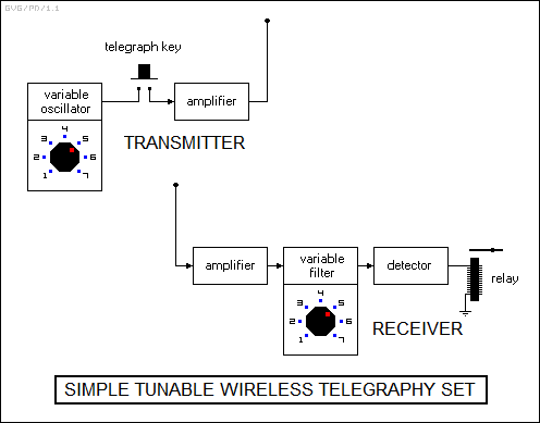
The problem with this simple scheme was that the transmitter generated waves over a wide and indiscriminate range of frequencies, with a single receiver picking up and mixing up transmissions from every transmitter in the line of sight. This problem was solved by fitting each transmitter with a "variable oscillator" -- an electronic circuit that generated electrical signals at different frequencies, as set by a knob turned by the transmitter operator. A receiver picked up this signal with its antenna, with the signal run through a "variable filter" -- an electric circuit consisting of an inductor coil and a variable capacitor that could be set by a knob to block out all frequencies except one.
This scheme allowed multiple transmitters to operate in a given area without interference. The transmitter operator set the transmitter oscillator to a given frequency or "channel", and then used a telegraph key to gate the oscillator output on and off into an amplifier circuit, which drove a high-power signal out of the antenna. The receiver operator set the receiver filter to the same channel. The receiver picked up radio waves on all frequencies and amplified them. The amplified received signal was run through the variable filter, and then into a "detector" circuit to convert high-frequency signals into a direct-current signal to activate the relay switch.
The detector included a "rectifier", a one-way valve for electricity, that eliminated half the waveform, with this rectified signal then passed through a "low pass filter", consisting in the simplest case of a resistor and a capacitor, that smoothed the received signals into pulses. The block diagram below gives a simple representation of such a system, For simplicity, the transmitter and receiver in the diagram can only be set to one of seven specific frequencies -- an unrealistically small range.
* This is obviously the same concept that is used in tuning a modern voice radio to different channels, though a voice radio works somewhat differently from a radio telegraph. In a simple "amplitude modulated" voice radio, the voice of a user is converted into an electrical waveform that controls or "modulates" the amplitudes or "envelope" of a variable oscillator signal. The modulated signal is then amplified and transmitted over an antenna. The oscillator frequency is known as the "carrier" frequency, since it "carries" the audio signal.
A receiver picks up the signal with its antenna, using a variable filter to isolate the desired channel. The signal is then amplified and passed through a detector circuit to extract the original audio signal. The audio signal is amplified and driven to a loudspeaker.
A radio channel is actually not a single frequency, but a range of frequencies. Although the details are beyond the scope of this simple document, the frequency range or "bandwidth" of a channel is roughly proportional to the amount of information carried by the channel. In the case of an audio broadcast, the bandwidth is a factor of the range of audio frequencies transmitted. That means that as a rule, a hi-fidelity audio transmission will take up more bandwidth than a low-fidelity transmission.
* The audio receiver described above will work, but in practice it doesn't work well for producing channels at high frequencies. In practice, most modern radio receivers use a "superheterodyne" scheme, in which the received signal picked up by the antenna and amplified is then run through a "mixer" or "heterodyne" circuit that combines the received signal with a lower fixed "intermediate frequency (IF)" signal produced by an oscillator. The mixer effectively subtracts the IF signal from the input signal, resulting in a low frequency modulated signal that is then detected and driven out the loudspeaker.
* The main problem with amplitude modulation is that most sources of environmental noise cause changes in the amplitude of a signal, introducing static and distortion. In addition, multiple signals on the same band will simply add to each other, with the receiver picking up both at the same time. This is actually an advantage in some circumstances, for example allowing multiple police cars to monitor each other's conversations, but it can be a nuisance in other circumstances.
The solution is what is known as "frequency modulation (FM)", in which the audio signal is mixed with the modulating signal to cause changes in frequency, not in amplitude. The rest of the stages of the transmitter are not conceptually different from those of an AM radio, and the receiver isn't much different either -- except that the simple detector circuit is replaced by some class of frequency-to-voltage converter circuit to extract the signal. FM is more noise-immune because there are relatively few forms of FM noise; and it is less prone to interference from other signals, because the strongest FM signal completely masks out weaker ones.
* An old-fashioned analog television signal was conceptually much the same as a voice radio. The TV sound track was transmitted with FM, while the basic visual signal, which was always in black and white, was transmitted by AM. A separate color signal was sent that "painted" colors, at lower resolution, on top of the basic black and white signal, with various schemes being used in various countries. Incidentally, this division of labor between the black and white signal and the color signal was the result of the fact that early on, broadcast TV was black and white, and when color was introduced there was a need to ensure that the broadcast signals could still be used by black and white sets.
Of course, since a moving picture generally contained more information than an audio signal, a TV signal required more bandwidth than an ordinary audio signal. Analog TV has now been replaced by digital broadcast systems, in which the signals are transmitted in the form of a stream of coded binary number values encoding the video and audio signals.
* Transmitter output power is measured in watts, or (as far as radar is concerned) more usually kilowatts (kW, thousands of watts) and megawatts (MW, millions of watts). Receiver "sensitivity", or the ability of the receiver to amplify received signals, is determined in terms of "decibels", defined as:
decibels = 10 * LOG10( output_power / input_power )
The amplification factor is commonly referred to as "gain".
A radio receiver, particularly one that is built into an automobile and is moving around, may be picking up a transmitter signal that varies in strength. That means that the volume of the radio output will tend to fade or grow continuously, requiring the listener to keep adjusting the volume control. A circuit known as an "automatic gain control (AGC)" helps correct this problem by measuring the average received power of the signal and adjusting the receiver gain to ensure that it stays as constant as possible.
BACK_TO_TOP* A transmitter needs an antenna to send its radio signal, and a receiver needs an antenna to pick up that radio signal. The simplest form of antenna is the "dipole". Suppose the electrical output of an oscillator is directed down two conductors, not connected at the ends. This will radiate EM energy from the open-circuit ends. It radiates energy much more effectively if the conductors are bent at the ends to form a right angle, with each bend being a quarter-wavelength long relative to the oscillator output.
This is a "half-wave" dipole. It is not only effective in generating radio waves at a particular frequency, it is also effective in picking them up. This is true in general of all antennas: they are "reciprocal", working much the same in transmission or reception, just in different directions. A single conductor can be used as well; this is the "monopole" antenna used in portable radio receivers and the like.
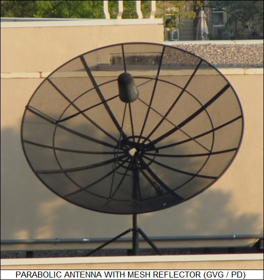
By itself, a dipole or monopole antenna "broadcasts" in all radial directions evenly, or in other words it is an "omnidirectional" antenna. It could be turned into a "directional" antenna by placing it in the center of a metal parabolic dish, with a small reflector above the dipole to bounce the signal back into the dish for transmission in one direction. However, instead of a dipole radio energy is usually just dumped into the dish through a "horn". It's really very much the same as using a parabolic mirror to focus light, only the wavelength of radio signals is longer.
While parabolic dishes are usually circular, creating a focused "pencil" beam, elliptical or cylindrical dishes with parabolic curvature can also be used if the radio beam needs to be focused along one axis but not along the other, or in other words has a "fan" configuration. The beam width is normally defined by a "3 dB" law, with the boundary of the beam defined as the surface where the power of the beam at the center falls by 3 dB.
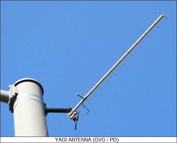
Another simple way to create a "directional" antenna with a dipole is to mount it within a row of parallel conductive rods, with the rods of decreasing length to the "front" of the dipole (relative to the direction of focus) and of increasing length to the "back" of the dipole. This type of antenna is known as a "Yagi-Uda" or just "Yagi" antenna. Such antennas are referred to as "end-fire antennas", since they are directional along their long axis. Dipole antennas, in contrast, are directional at a right angle to their plane.
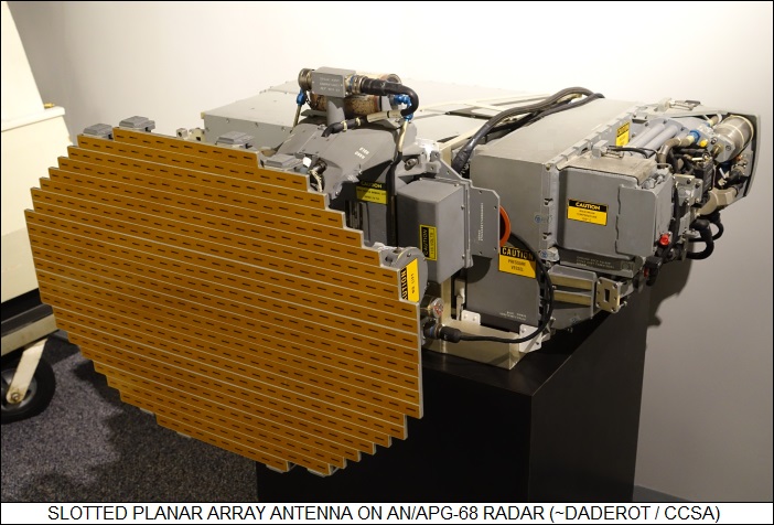
A more sophisticated approach is to obtain a directed focus by using an antenna with multiple dipoles in a grid arrangement, with the focus obtained by interference effects. Such "dipole arrays" were common with early longwave radars. Arrays can be made with end-fire antennas as well, and very significantly as slotted plates, with radio energy fed through the slots. The slots act as dipoles, though while the polarization of a radio wave generated by a dipole is in line with the long axis of the dipole, it's at a right angle to the long axis of the slot. Slotted planar arrays are popular these days, since shrewd slot arrangements allow them to be much more efficient than simple parabolic antennas, which will waste about two-thirds of the energy pumped into them. A well-designed slotted planar array will waste less than a third of the energy.
* Directional antennas are characterized by a factor known as "antenna gain". This is simply the ratio of the focused beam power to the same broadcast power sent through an omnidirectional antenna. For example, if the focused beam has 50 times the power of an omnidirectional antenna with the same transmitter power, the directional antenna has a gain of 50, or 17 dB.
The larger the receiver dish, the greater the receiver sensitivity, since it creates a bigger "bucket" or "eye" to collect radio waves. However, the longer the wavelength, the bigger the dish has to be to focus the radio waves, and conversely the more focused the beam, the bigger the antenna. One simple rule of thumb gives the width of the antenna as:
width_in_meters = 51 * wavelength_in_meters / beamwidth in degrees
For example, to obtain a beamwidth of 2 degrees at a low frequency of 5 MHz (corresponding to 60 meters), the antenna width is:
51 * 60 / 2 = 1,530 meters
This is not a reasonable size for an antenna. At 150 MHz, with a wavelength 30 times shorter, the antenna size shrinks to 51 meters, and at 1 GHz, with a wavelength 200 times shorter, the antenna size shrinks to 7.65 meters. Big antennas don't necessarily mean high power or sensitivity: they may indicate low frequency operation, or narrow beamwidths, or both.
Another minor related fact is that the dish doesn't have to be solid. It can be a mesh, just as long as the mesh grid spacing is less than that of the radar operating wavelengths. This makes for a lighter antenna, and also one not so easily disturbed by the wind.
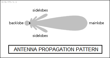
* Directional antennas don't always generate all their radio output in a nice neat directional beam. Interference between transmit signals may generate "sidelobes" that cause unwanted transmissions to the sides of the beam, or a "backlobe" in the reverse direction. The sidelobes and backlobe can rob the main lobe of energy and of course corrupt the directionality of the beam, generating and receiving signals in unwanted directions. Proper antenna design minimizes the power lost by sidelobes and backlobes.
Sidelobes are a particular nuisance in radars, since they can produce false returns and can pick up radio interference, including deliberate interference produced by countermeasures systems. In radar systems, the ratio of sidelobe to main beam power is generally kept to less than -40 dB, or 1:10,000. This is done in arrays by carefully arranging the power levels of the array elements, with more power in the center elements than at the elements along the edge. There are a number of "aperture tapering" schemes to define the proper arrangements of power levels.
BACK_TO_TOP* The best way to explain radar is to imagine standing on one side of a canyon, and shouting in the direction of the distant wall of the canyon. After a few moments, an echo will come back. The length of time it takes an echo to come back is directly related to how far away the distant canyon wall is. Double the distance, and the length of time doubles as well. Given that the speed of sound is about 1,200 KPH (745 MPH) at sea level, then timing the echo with a stopwatch will give the distance to the remote canyon wall. If it takes four seconds for the echo to come back, then since sound travels about 330 meters (1,080 feet) in a second, the distance is about 660 meters (2,160 feet).
Radar uses exactly the same principle, but it times echoes of radio or microwave pulses and not sound. Like a wireless telegraphy set, a simple radar has a transmitter and a receiver, with the transmitter sending out pulses, short bursts, of EM radiation and the receiver picking them up.
In the case of the radar, the receiver is picking up echoes from a distant target, with the echoes timed to determine the distance to the target. Early radars simply used an oscilloscope to perform the timing, with the detected return signal fed into the oscilloscope as a "video" signal, and showing up as a peak or "blip" on the display.
An oscilloscope measures an electrical signal on an electronic beam that moves or "sweeps" from one side of a display to the other at a certain rate. The rate is determined by a "timebase" circuit in the oscilloscope. For example, the sweep rate might push the sweep from one side of the display to the other in a millisecond (thousandth of a second). If the display were marked into ten intervals, that would mean the sweep would pass through each interval in 0.1 milliseconds. While this would be shorter than the human eye could follow, the sweep is normally generated repeatedly, allowing the eye to see it.
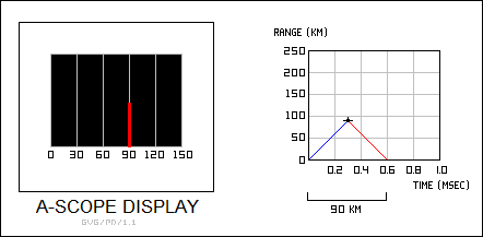
Since EM radiation propagates at 300,000,000 meters per second, or 300,000 meters per millisecond, then each 0.1 millisecond interval would correspond to 30,000 meters, or 30 kilometers (18.6 miles). If the sweep on the scope is "triggered" to start when the radar transmitter sends out the radio pulse, and the sweep displays a blip on the sixth interval on the display, then the pulse has traveled a total of 180 kilometers (112 miles). Since this is the round-trip distance for the pulse, that means that the target is 90 kilometers (56 miles) away. The trigger signal provides synchronization, so it can be regarded as a type of "synch" or "sync" signal. The sweep is called a "range sweep" and the output of the display is called a "range trace".
The display scheme described here is known as an "A-scope", and allows the user to determine the range to a target. A simple representation of an A-scope is shown below, along with a graph plotting the travel of the pulse with respect to time:
The amplitude of the return also gives some indication of the size of the target, though the relation between return amplitude and target size is not straightforward, as discussed later.
* It would also be nice to know what the direction to the target is, in terms of its "altitude (vertical direction)" and "azimuth (left to right direction)".
This is a bit trickier to describe, but no more complicated in the end. Some early radars, like the famous British "Chain Home" sets that helped win the Battle of Britain, simply transmitted radio waves from high towers in a flood over their field of view, and used a directional receiver antenna to determine the direction of the echo. Chain Home actually used a scheme where the power of the echo was compared at separated receiver antennas to give the direction which, astoundingly, worked reasonably well. Other such "floodlight" radars used directional receiver antennas that could be steered to identify the direction of the echo. Incidentally, a radar that uses receive and transmit antennas sited in different locations is known as a "bistatic", or in the more general case "multistatic", radar.
Floodlight radars were quickly abandoned. They spread their radio energy over a wide area, meaning that any echo was faint, and so range was limited. The next step was to make a radar with a steerable transmitter antenna. For example, two directional antennas, one for the transmitter and the other for the receiver, could be ganged together on a steerable mount and pointed like a searchlight, an arrangement that is sometimes called "quasi-monostatic". The transmitter antenna generated a narrow beam, and if the beam hit a target, an echo would be picked up by the receiving antenna on the same mount. The direction of the antennas naturally gave the direction to the target, at least to an accuracy limited by the width in degrees of the beam, while the distance to the target was given by the trace on the A-scope.
Of course, it was realized early on that it would be more economical and less physically cumbersome to use one antenna for both transmit and receive instead of separate antennas; it was possible to do so in theory because a radar transmits a pulse, then waits for an echo, meaning it doesn't transmit and receive at the same time. The problem in practice was that the receiver was designed to listen for a faint echo, while the transmitter was designed to send out a powerful pulse. If the receiver was directly linked to the transmitter when a pulse was sent out, the transmit pulse would fry the receiver.
The solution to this problem was the "duplexer", a circuit element that protected the receiver, effectively becoming an open connection while the transmit pulse was being sent, and then closing again immediately afterward so that the receiver could pick up the echo. This was done with certain types of gas-filled tubes, with the output pulse ionizing the gas and making the tube nonconductive, and the tube recovering quickly after the end of the pulse. More sophisticated duplexer schemes would be developed later. The receiver was also generally fitted with a "limiter" circuit that blocked out any signals above a certain power level. This prevented, say, transmissions from another nearby radar from destroying the receiver.
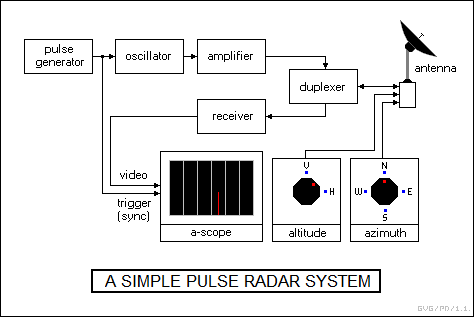
* After this evolution of steps, the result is a simple, workable radar. It has a single, steerable antenna that can be pointed like a searchlight. The antenna repeatedly sends out a radio pulse and picks up any echoes reflected from a target. An A-scope display gives the interval from the time the pulse is sent out and the time the echo is received, allowing the operator to determine the distance to the target.
The transmitter emits pulses on a regular interval, typically a few dozen or a few hundred times a second, with the A scope trace triggered each time the transmitter sends out a pulse to display the receiver output. The number of pulses sent out each second is known as the "pulse repetition rate" or more generally as the "pulse repetition frequency (PRF)", measured in hertz.
The width of a radar pulse is an important but tricky consideration. The longer the pulse, the more energy sent out, improving sensitivity and increasing range. Unfortunately, the longer the pulse, the harder it is to precisely estimate range. For example, a pulse that last 2 microseconds is 600 meters (2,000 feet) long, and in that case there is no real way to determine the range to an accuracy of better than 600 meters, and there is also no way to track a target that is closer than 600 meters. In addition, a long pulse makes it hard to pick out two targets that are close together, since they show up as a single echo.
PRF is another tricky consideration. The higher the PRF, the more energy is pumped out, again improving sensitivity and range. The problem is that with a simple radar it makes no sense to send out pulses at a rate faster than echoes come back, since if the radar sends a pulse and then gets back an echo from an earlier pulse, the operator is likely to be confused by the "ghost echo". This is usually not too much of a problem, since a little quick calculation shows that even a PRF of 1,000 gives enough time to get an echo back from 150 kilometers (95 miles) away before the next pulse goes out. However, as mentioned above, propagation of radar waves can be freakishly affected by atmospheric conditions that create ducting or other unusual phenomena, and sometimes radars can get back echoes from well beyond their design range.
This can be confusing, because a pulse will be sent out and a return will be received very quickly, indicating that the target is close. In reality, the target is distant and the return is from the previous pulse. This is called a "second time around" return. Given a PRF of 1,000, then a target 210 kilometers (130 miles) away will appear to be only 60 kilometers (37 miles) away. Similar confusions could be caused by returns that arrive from long ranges after more than one additional pulse, resulting in "multiple time around" returns. Of course, a simple pulse radar also has "blind ranges" or "blind zones": if our example radar is trying to spot a target exactly 150, 300, or 450 kilometers away, the return will arrive when the next pulse is being sent out and the radar will never spot it.
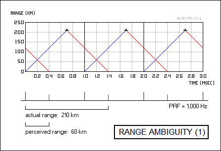
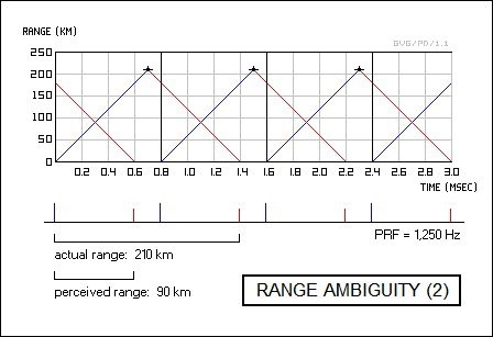
To deal with such "range ambiguities", radars were designed so they could be switched between different PRFs. Switching from one PRF to another would not affect a "first time around" echo, since the delay from pulse output to pulse reception would remain the same, but the switch would make a ghost return from a current pulse jump on the display. Suppose our radar could be switched from a PRF of 1,000 Hz to 1,250 Hz, and is trying to track a target 210 kilometers away. At 1,000 Hz, the maximum range is 150 kilometers and the target appears to be 60 kilometers away, but at 1,250 Hz the maximum range is 120 kilometers (75 miles) and the target return jumps to a perceived range of 90 kilometers (56 miles). The fact that the target range jumps when PRF is changed reveals the range ambiguity; adding perceived range to the maximum range for each PRF setting gives the actual range.
* Incidentally, the power of the transmitter pulse is given as "peak power", usually in kilowatts or megawatts. This may be an impressive value, but it's only the power that goes into the pulse itself. Suppose we have a pulse width of 2 microseconds with a peak power of 150 kilowatts. If we have a PRF of 500, then the time from pulse to pulse, or "pulse period", is 1/500 = 2 milliseconds, or two thousandths of a second. This means that the average power transmitted by our radar is only:
150 kW * ( 2 microseconds / 2 milliseconds) = 0.15 kW = 150 watts
-- which is about as much as the power draw of a bright old-fashioned household incandescent light bulb.
* One of the first US early warning radars, the "SCR-27O", provides a good example of such a simple radar. It was a VHF radar, actually operating at what by modern standards at a low frequency / long wavelength of 100 MHz / 3 meters. It had a steerable rectangular "flyswatter" style dipole array of 4 x 8 dipoles, and featured a pulse width of 10 to 25 microseconds, a PRF of 621 Hz, and a peak power of 100 kW.
BACK_TO_TOP* Early radars were based on traditional vacuum-tube technology. The basic classic vacuum tube was the "triode", which consisted of a vacuum-sealed tube with plates at each end and a mesh or "grid" of wires in the middle, with each of the three connected to its own external lead. The "cathode" plate at one end was negatively charged and heated by a separate filament, to boil off electrons that were attracted to the positively-charged "anode" plate at the other end. If the grid was given a negative voltage, it could shut off the flow of electrons; in this way, a low-power signal fed to the grid of a triode could modulate the flow of electrons through the tube, creating the same signal at a significantly boosted power level.
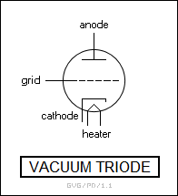
Such vacuum tubes were used to construct amplifier and oscillator circuits for radars, an oscillator in this case being nothing more than an amplifier with some of its output fed back out-of-phase to its input through a filter circuit designed to pass the desired frequency. High-power triodes, sometimes with liquid cooling, were used for the high-power radar transmitter output stages. Triodes were an effective technology, but could not produce very high frequencies.
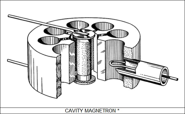
* Higher frequencies, in the microwave range, could produce more focused beams with greater resolution. They were produced by a wartime invention, the "cavity magnetron". It was actually invented roughly in parallel in a large number of countries, but the British ran with it and also passed it on to the US. It is still in widespread use, at least in microwave ovens.
The core of the magnetron is a metal cylinder, not so different in appearance from the cylinder of a revolver-type pistol. The center of the cylinder is bored out, and a set of "cavities" are bored through the cylinder around the central hole. Each cavity is connected to the central hole through a slot. A conductive rod is placed in the central hole, to act as the negatively charged cathode, while the cylinder itself acts as the positively charged anode. The assembly is sealed inside a vacuum envelope, and magnets are placed top and bottom.
Electrons move at a right angle to a magnetic field, and so the magnets cause the electrons moving from cathode to anode to swirl around the cathode rod in a spiral. Electrons emit EM radiation when they are accelerated, and so as they are pulled around the cathode they emit EM radiation over a wide range. This radiation flowed into the cavities around the central shaft. The cavities act as "resonant chambers", with EM radiation of a specific wavelength building up inside them. The wavelength in practice is about 8 times the diameter, or a 1.2 centimeter cavity would produce a 10 centimeter / 3 GHz signal. One of these resonant cavities is tapped out to drive microwave power to the radar system.
The magnetron's operating wavelength can be adjusted within a limited range by lowering a set of slugs into the cavities to adjust their resonant frequency. Unlike the vacuum triode, the magnetron is not an amplifying device as such: it generates its own high-power signal at a set frequency. Initially, the rest of the radar still remained reliant on vacuum tubes.
Incidentally, at lower frequencies it is possible to generate a signal in the oscillator subsystem and send it to an antenna over a solid-wire connection, usually in the form of "coaxial cables" -- consisting of a central core conductor surrounded by an insulator and then a conductive wrapper, where it excites a dipole or similar element to generate radio waves. Trying to send an electrical signal over a solid conductor is more difficult at higher frequencies, resulting in losses, so the radio energy is produced directly by the oscillator and "piped" down hollow tubes with conductive walls, known as "waveguides", to an antenna feed horn.
BACK_TO_TOP* The tools provided so far give enough information for understanding the "radar range equation", the most fundamental formula for radar operation. As its name implies, it gives the possible maximum range of a radar, as determined by the following factors:
This gives a simplified version of the radar range equation:
     power * gain * RCS
   -----------------------  >  noise
    attenuation * range^4
There are many variations of this equation, usually providing greater detail or modified to demonstrate the capabilities of different radar configurations. The basic idea is simple: the capability of a radar to detect a target is directly proportional to its transmit power, its receiver gain, and the RCS of a target; and inversely proportional to the atmospheric attenuation and the fourth power of the range.
BACK_TO_TOP* The simple pulse radar described above was actually preceded in the prewar timeframe by simpler systems that consisted of a transmitter sending a signal to a receiver on a continuous basis. For example, the transmitter could be placed on one side of the mouth of a harbor and the receiver placed on the other, with a ship entering the harbor breaking the radio beam and announcing its presence. The transmitter and receiver could also be placed on the same side of the harbor, with the passing ship bouncing the radio beam back to the receiver. These simple "continuous wave (CW)" systems weren't really radars since they couldn't realistically give a range to a target, they could only detect that something was there. They are better described as "CW alarm systems", and they are really something of a footnote in the history of radar.
However, although a simple CW alarm can't determine range, a direct variation on it can be used to determine velocities. Suppose a continuous radio signal at a given frequency is focused on an aircraft approaching head-on; the velocity of the aircraft will actually increase the frequency of the echo. If the aircraft is going directly away, it will decrease the frequency of the echo return. This is known as the "Doppler shift". The same effect is observed with sound waves when an aircraft is flying overhead: as it approaches, the sound of the aircraft has a high pitch, in other words a high audio frequency, and when it is going away it has a low pitch, or a low audio frequency.
Derivation of the Doppler shift is a bit beyond this document, but can be found in any simple physics text. For a radar, which generally tracks targets moving much slower than the speed of light, the shift in frequency, or "Doppler frequency" is roughly:
doppler_frequency = 2 * target_velocity / radar_wavelength
For example, if:
-- then the Doppler frequency is:
2 * 278 / 3 = 185 Hz
This is the shift up in frequency if the target is approaching and the shift down in frequency if the target is moving away. Incidentally, the Doppler shift for radio emissions transmitted from the target itself is only half this, 92.5 Hz; the value is doubled for radar because the target is moving as the radar arrives, causing a shift, and as the return is reflected, causing a second shift.
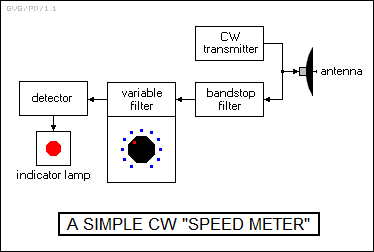
It would be possible to imagine a simple continuous-wave radar Doppler velocity meter, consisting of a transmitter unit and a receiver unit. Since this device is only intended to measure velocity, the two units can share the same antenna, with the receiver blocking out the signal of the transmitter with a "band rejection filter" that blocks signals at the transmit frequency but allows all others to pass. The transmitter would send a radio beam at a target. A calibrated dial on the receiver could then be used to adjust a variable filter until the Doppler-shifted echo was received and lit up an indicator light. The velocity could be read off the dial. Of course, this scheme only gives the velocity of the target on a straight-line radial to the detector. At any angle off the radial the perceived velocity is smaller, until at 90 degrees it falls to zero.
A more practical device would feature a receiver that had sets of fixed filters in a range of frequencies above and below the transmitter frequency. Each filter would be connected to a simple circuit that activated a light on the front panel of the receiver, with each light marked with a particular range of velocities. If the Doppler shifted echo passed through a specific filter, it would turn on the appropriate light to give the target velocity. The radars used by police to catch speeders actually operate more or less along such a principle, though their implementation is much more sophisticated, and they will actually give speed readings.
The essential point here is that, although timing radio pulses can be used to obtain ranges to targets, it is also useful to obtain information from the Doppler shift to learn about the velocities of targets. The combination of these two approaches in "pulse Doppler" radars is an important theme in modern radars and is discussed later.
BACK_TO_TOP